Introduction
The logistic sigmoid is one of the most popular activation functions used when working with the probability distributions associated with deep learning. It is a function that produces the \(\phi\) parameter of a Bernoulli distribution due to its finite range \((0,1\)), which is a valid range suitable for the values of the \(\phi\) parameter. A common use case for this function is in binary classification.
Some Mathematical description
A sigmoid function is a bounded, differentiable, real function that is defined for all real input values and has a non-negative derivative at each point and exactly one inflection point. -- Wikipedia
A sigmoid function is a mathematical function possessing a distinctive S-shaped curve or sigmoid curve.
Mathematically, this function is defined as:
$$ S(z) = \frac {1}{1+e^{-z}} = \frac {e^z}{e^z+1} = 1-S(-z) \tag{1} $$
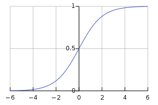
If we made a plot of the mathematical function given by equation 1, we would end up with a graph having a response value (y-axis) with range \((0,1\)):
 Fig. 1, Graphical representation of the sigmoid function[1].
N.B: Another commonly used response value range is \((-1,1\)).
The sigmoid function saturates when its argument has extreme values (positive or negative), resulting in a very flat function that is insensitive to minute changes in its input.
An area where the sigmoid function is flawed is evident in the Vanishing Gradient Problem experienced in deep neural networks, this happens during backpropagation and the sigmoid activation often encourages this phenomenon, because its derivative is less than 0.25 at all values of its argument, and is extremely small at saturation [2]. One of the solutions to this problem is using a different activation function called the ReLU function
As stated earlier, the sigmoid function has found an application in the field of artificial neural networks where one of its variants (the logistic sigmoid) is used as an activation function. It has a similar equation to that of the vanilla sigmoid function given by:
$$ \sigma(x) = \frac{1}{1 + e^{-x}} \tag{2} $$
And it maps a set of real numbers to a probability space which is super useful for binary classification tasks.
$$ (-\infty, \infty) \mapsto (0,1) \tag{3} $$
Remark: Other variants of the sigmoid function are the Hyperbolic tangent and the Arc-tangent
Coding up the Logistic sigmoid function
The definition of the sigmoid function makes it easy for us to implement in vanilla python or by using available frameworks such as Pytorch and Tensorflow. In this section, we show a hardcoded version of the logistic sigmoid function and its PyTorch and Tensorflow equivalents.
Python approach
>>> import numpy as np

# define the function
>>> def sigmoid(x):
        return 1/(1+np.exp(-x))

# use the function
>>> x = np.random.rand(10)
>>> sigmoid(x)
# output
>>> array([0.52267203, 0.64301185, 0.72775684, 0.71219049, 0.65616863,
           0.56483881, 0.53707694, 0.51163662, 0.64807105, 0.62321943])
PyTorch
>>> import torch

>>> m = torch.nn.Sigmoid()
>>> x = torch.rand(10)
>>> output = m(x)
# output
>>> tensor([0.7040, 0.6892, 0.5103, 0.5778, 0.5457, 0.5122, 0.7197,
            0.7098, 0.6918, 0.6192])
Tensorflow
>>> import tensorflow as tf

>>> g = tf.random.get_global_generator()
>>> x = g.normal(size=[10])
>>> sig_function = tf.math.sigmoid(x)
>>> sig_function
# output
>>> <tf.Tensor: shape=(10,), dtype=float32, numpy=
       array([0.72447205, 0.5554114 , 0.2537729 , 0.34373525, 0.5937648 ,
       0.43216416, 0.820067  , 0.09450763, 0.42425528, 0.5829959 ],
       dtype=float32)>
N.B: Instead of generating random numbers like I did in the examples above, you can create an input vector having constant values. This would return consistent values as output vectors.
Conclusion
This article introduced the concept of the sigmoid function and its application in artificial neural networks, highlighting some of its benefits and shortcomings. We then showed how to implement the sigmmoid function using vanilla python (we kind of borrowed numpy's exponential function 😉) and popular deep learning frameworks including PyTorch and Tensorflow. Hope you enjoyed it, and see you next time!
