Introduction

The rectified linear unit function, ReLU, is one of the three most commonly used activation functions used in deep learning, including the sigmoid (sig) and hyperbolic tangent (tan) functions. It is a type of ramp function that is somewhat analogous to the half-wave rectification principle in electrical engineering.

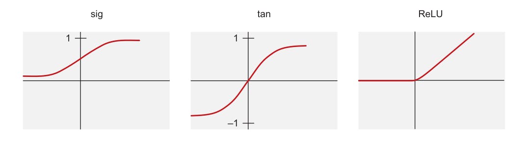Fig. 1. Activation functions [1]

The ReLU Function

The ReLU function began to surface in the context of visual feature extraction in hierarchical neural networks starting in the late 1960s. Arguments later emerged about it having strong biological motivations and mathematical justifications. One reason for its acceptance over other activation functions like the logistic sigmoid (an activation function based on probability theory) and its hyperbolic tangent equivalent is due to the fact that it was found to enable better training of deeper networks. Currently, the ReLU function is arguably the most used activation function in deep learning.

A ReLU activation unit is known to be less likely to create a vanishing gradient problem because its derivative is always 1 for positive values of the argument. -pg 44, Neural Networks and Deep Learning 2018

Traditionally, the sigmoid and tanh activations were the most popular choices in the hidden layers, but the ReLU activation has become increasingly popular in recent years because of the desirable property that it is better at avoiding the vanishing and exploding gradient problems, -pg 62, Neural Networks and Deep Learning 2018

Advantages

The ReLU activation function benefits greatly from sparsity (a topic beyond the scope of this article), which it uses to allow a network to easily obtain sparse representations. For example, in a randomly initialized network, around 50% of hidden units are activated (have a non-zero output). This leads to linear computations on subsets of neurons, and a more fluid flow of gradients on the active parts of neurons (hence eliminating the gradient vanishing effect due to activation non-linearities of sigmoid or tanh units). As a result, mathematical investigations are easier and computations are cheaper [2].

For more information, check out the paper on Deep Sparse Rectifier Neural Networks

Let's introduce some interesting mathematics

In the previous section, we defined the ReLU function as some kind of ramp function. In mathematics, this type of function is widely known as the positive part and is given by the equation:

$$ \begin{equation} f^+(x) = \max(f(x),0) = \begin{cases} f(x) & \text{if}\ f(x) \gt 0 \\ 0, & \text{otherwise} \end{cases} \tag{1} \end{equation} $$

And we can generalize equation \(1\) to define the ramp function given by:

$$ \mathbf R := \max(x, 0) \tag{2} $$

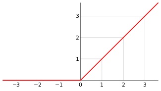Fig. 2. Graphical representation of the ramp function [3]

Remark: intuitively, we graph \(f^+\) by taking the graph of \(f\), eliminating the part under the x-axis, and letting \(f^+\) take the value zero there.

For the ReLU activation function, it is mathematically defined as the positive part of its argument, given by:

$$ f(x) = x^+ = \max(0,x) \tag{3} $$ Where \(x\) is the input to a neuron.

From equations \(2\ \text{and}\ 3\) we can see the similarities between the ramp function and the ReLU function, and that is why the graphical representation of the ReLU function assumes the same shape as that of the ramp function.

Coding up the ReLU Function

Finally, we're at the interesting part! 😎 The mathematical definition of the ReLU function makes it easy to implement in terms of codes, and we can compute it by writing a simple conditional statement, or using the \(max()\) function in python. This section shows both methods, so let's get to it!

Using conditionals

>>> def ReLU(x): 
        if x > 0 or x == 0:
            return x
        else:
            return 0

>>> ReLU(100)
# Returns
>>> 100
>>> ReLU(-100)
# Returns 
>>> 0

Using the \(max()\) function in Python

>>> def ReLU(x):
        return max(0, x)

>>> ReLU(100)
# Returns 
>>> 100
>>> ReLU(-100)
# Returns
>>> 0

In practice, there is rarely a need for you to hard-code activation functions for any given task since there are available libraries that provide such functions, neither of the hard-coded functions provided above will generalise for an input of arrays, so it is best to use libraries like Pytorch and Tensorflow. We show how to compute the ReLU activation function using either of these libraries below.

Using Tensorflow/Keras

>>> import tensorflow as tf

>>> arr = tf.constant([-10, -5, 0.0, 5, 10], dtype = tf.float32)
>>> tf.keras.activations.relu(arr).numpy()

# Returns
>>> array([ 0.,  0.,  0.,  5., 10.], dtype=float32)

Using Pytorch

>>> import torch
>>> import numpy as np

>>> m = torch.nn.ReLU()
>>> arr = np.array([-10, -5, 0.0, 5, 10])
>>> t_arr = torch.tensor(arr) # convert numpy array to tensor
>>> relu = m(t_arr)
>>> print(relu)

# Returns 
>>> tensor([ 0.,  0.,  0.,  5., 10.], dtype=torch.float64)

Remark: Across all methods, notice how the ReLU function handles values less than or equal to zero... it returns them as zero!

When we plot either of the outputs from the Tensorflow or Pytorch approach, we obtain a graph similar to the one given in fig 2.

>>> import matplolib.pyplot as plt
>>> plt.style.use("seaborn")

# Using the output from our Pytorch implementation 
>>> plt.plot(relu)
>>> plt.show()

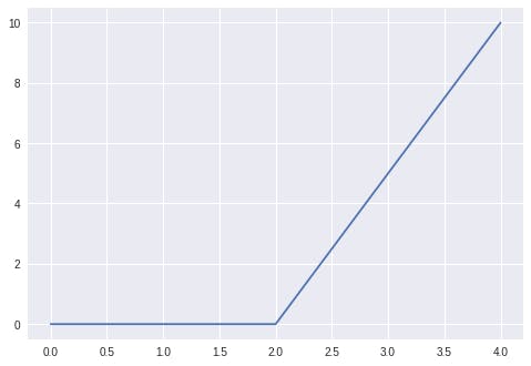Fig. 3. Graph of the Pytorch output of the ReLU function.

Conclusion

In this article, we introduced the ReLU activation function and defined a few interesting concepts, verified that it is essentially a ramp function, and showed how to implement the function using python... I hope you enjoy reading it as much as I enjoyed writing it. See you next time!

References

[1] Machine Learning With Tensorflow 2nd Edition

[2] Deep Sparse Rectifier Neural Networks

[3] Ramp Function